3.matplotllib
joker ... 2022-4-7 大约 9 分钟
# 3.matplotllib
# 3.1 基本用法
import matplotlib.pyplot as plt
import pandas as pd
import numpy as np
x=np.linspace(-1,1,50)
y=2*x+1
plt.plot(x,y)
plt.show()
1
2
3
4
5
6
7
2
3
4
5
6
7
# 3.2 figure 用法
每一个figure 中,就会有不同的图片
import matplotlib.pyplot as plt
import pandas as pd
import numpy as np
x=np.linspace(-1,1,50)
y1=2*x+1
y2=x**2
plt.figure()
plt.plot(x,y1)
plt.show()
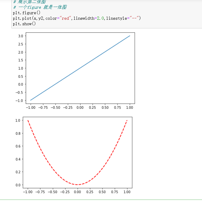
# 展示第二张图
# 一个figure 就是一张图
plt.figure()
plt.plot(x,y2,color="red",linewidth=2.0,linestyle="--")
plt.show()
1
2
3
4
5
6
7
8
9
10
11
12
13
14
15
2
3
4
5
6
7
8
9
10
11
12
13
14
15
# 3.3 设置坐标轴
import matplotlib.pyplot as plt
import pandas as pd
import numpy as np
x=np.linspace(-3,3,50)
y1=2*x+1
y2=x**2
plt.figure()
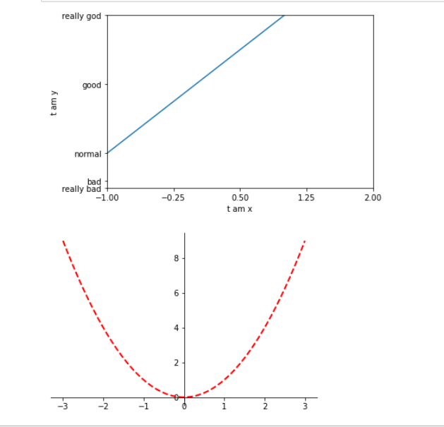
plt.xlim((-1,2))
plt.ylim((-2,3))
plt.xlabel("t am x")
plt.ylabel("t am y")
new_ticks=np.linspace(-1,2,5)
plt.xticks(new_ticks)
plt.yticks([-2,-1.8,-1,1,3],["really bad","bad","normal","good","really god"])
plt.plot(x,y1)
plt.show()
plt.figure()
# 移动x 轴或者y 轴
ax=plt.gca()
ax.spines["right"].set_color("none")
ax.spines["top"].set_color("none")
ax.xaxis.set_ticks_position("bottom")
ax.yaxis.set_ticks_position("left")
ax.spines["bottom"].set_position(("data",0))
ax.spines["left"].set_position(("data",0))
plt.plot(x,y2,color="red",linewidth=2.0,linestyle="--")
plt.show()
1
2
3
4
5
6
7
8
9
10
11
12
13
14
15
16
17
18
19
20
21
22
23
24
25
26
27
28
2
3
4
5
6
7
8
9
10
11
12
13
14
15
16
17
18
19
20
21
22
23
24
25
26
27
28
# 3.4 图例
import matplotlib.pyplot as plt
import pandas as pd
import numpy as np
x=np.linspace(-3,3,50)
y1=2*x+1
y2=x**2
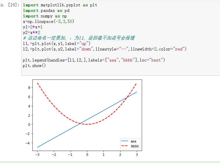
# 这边命名一定要加, ,为l1, 返回值不加逗号会报错
l1,=plt.plot(x,y1,label="up")
l2,=plt.plot(x,y2,label="down",linestyle="--",linewidth=2,color="red")
plt.legend(handles=[l1,l2,],labels=["aaa","bbbb"],loc="best")
plt.show()
1
2
3
4
5
6
7
8
9
10
11
12
2
3
4
5
6
7
8
9
10
11
12
# 3.5 标注
s 为注释文本内容
xy 为被注释的坐标点
xytext 为注释文字的坐标位置
xycoords 参数如下:
- figure points:图左下角的点
- figure pixels:图左下角的像素
- figure fraction:图的左下部分
- axes points:坐标轴左下角的点
- axes pixels:坐标轴左下角的像素
- axes fraction:左下轴的分数
- data:使用被注释对象的坐标系统(默认)
- polar(theta,r):if not native ‘data’ coordinates t
weight 设置字体线型
{‘ultralight’, ‘light’, ‘normal’, ‘regular’, ‘book’, ‘medium’, ‘roman’, ‘semibold’, ‘demibold’, ‘demi’, ‘bold’, ‘heavy’, ‘extra bold’, ‘black’}
color 设置字体颜色
- {‘b’, ‘g’, ‘r’, ‘c’, ‘m’, ‘y’, ‘k’, ‘w’}
- ‘black’,'red’等
- [0,1]之间的浮点型数据
- RGB或者RGBA, 如: (0.1, 0.2, 0.5)、(0.1, 0.2, 0.5, 0.3)等
arrowprops #箭头参数,参数类型为字典dict
- width:箭头的宽度(以点为单位)
- headwidth:箭头底部以点为单位的宽度
- headlength:箭头的长度(以点为单位)
- shrink:总长度的一部分,从两端“收缩”
- facecolor:箭头颜色
bbox给标题增加外框 ,常用参数如下:
- boxstyle:方框外形
- facecolor:(简写fc)背景颜色
- edgecolor:(简写ec)边框线条颜色
- edgewidth:边框线条大小
import matplotlib.pyplot as plt
import numpy as np
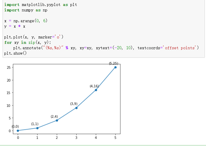
x = np.arange(0, 6)
y = x * x
plt.plot(x, y, marker='o')
for xy in zip(x, y):
plt.annotate("(%s,%s)" % xy, xy=xy, xytext=(-20, 10), textcoords='offset points')
plt.show()
1
2
3
4
5
6
7
8
9
10
2
3
4
5
6
7
8
9
10
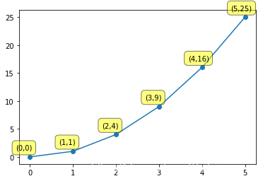
例二
import matplotlib.pyplot as plt
import numpy as np

x = np.arange(0, 6)
y = x * x

plt.plot(x, y, marker='o')
for xy in zip(x, y):
    plt.annotate("(%s,%s)" % xy, xy=xy, xytext=(-20, 10), textcoords='offset points',
    bbox=dict(boxstyle='round,pad=0.5', fc='yellow', ec='k', lw=1, alpha=0.5)
plt.show()
1
2
3
4
5
6
7
8
9
10
11
2
3
4
5
6
7
8
9
10
11
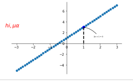
例三
import matplotlib.pyplot as plt
import pandas as pd
import numpy as np
x=np.linspace(-3,3,50)
y1=2*x+1
y2=x**2
plt.scatter(x,y1)
plt.figure(num=1,figsize=(8,5))
ax=plt.gca()
ax.spines["right"].set_color("none")
ax.spines["top"].set_color("none")
ax.xaxis.set_ticks_position("bottom")
ax.yaxis.set_ticks_position("left")
ax.spines["bottom"].set_position(("data",0))
ax.spines["left"].set_position(("data",0))

x0=1
y0=2*x0+1
plt.scatter(x0,y0,s=50,color='b')
plt.plot([x0,x0],[y0,0],"k--",lw=2.5)
# xytext 就是文字偏离点的位置
plt.annotate(r"$2x+1=%s$" % y0,
             xy=(x0,y0),
             xycoords="data",
             xytext=(+30,-30),
             textcoords="offset points",
             fontsize=6,
             arrowprops=dict(arrowstyle="->",connectionstyle="arc3,rad=.2")
             )

plt.text(-3.7,3,r"$hi ,\mu \alpha$",fontdict={"size":16,"color":"r"})

plt.show()
1
2
3
4
5
6
7
8
9
10
11
12
13
14
15
16
17
18
19
20
21
22
23
24
25
26
27
28
29
30
31
32
33
2
3
4
5
6
7
8
9
10
11
12
13
14
15
16
17
18
19
20
21
22
23
24
25
26
27
28
29
30
31
32
33
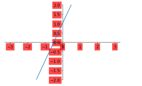
# 3.6 能见度
import matplotlib.pyplot as plt
import pandas as pd
import numpy as np
x=np.linspace(-3,3,50)
y1=2*x+1
y2=x**2
plt.plot(x,y1)
plt.figure(num=1,figsize=(8,5))
plt.ylim(-2,2)
ax=plt.gca()
ax.spines["right"].set_color("none")
ax.spines["top"].set_color("none")
ax.xaxis.set_ticks_position("bottom")
ax.yaxis.set_ticks_position("left")
ax.spines["bottom"].set_position(("data",0))
ax.yaxis.set_ticks_position("left")
ax.spines["left"].set_position(("data",0))

for label in ax.get_xticklabels()+ax.get_yticklabels():
    label.set_fontsize(12)
    label.set_bbox(dict(facecolor="red",edgecolor="None",alpha=0.7))

plt.show()
1
2
3
4
5
6
7
8
9
10
11
12
13
14
15
16
17
18
19
20
21
22
23
2
3
4
5
6
7
8
9
10
11
12
13
14
15
16
17
18
19
20
21
22
23
# 3.7 各种图
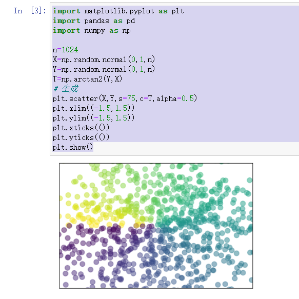
# 3.7.1 散点图
import matplotlib.pyplot as plt
import pandas as pd
import numpy as np

n=1024
X=np.random.normal(0,1,n)
Y=np.random.normal(0,1,n)
T=np.arctan2(Y,X)
# 生成
plt.scatter(X,Y,s=75,c=T,alpha=0.5)
plt.xlim((-1.5,1.5))
plt.ylim((-1.5,1.5))
plt.xticks(())
plt.yticks(())
plt.show()
1
2
3
4
5
6
7
8
9
10
11
12
13
14
15
2
3
4
5
6
7
8
9
10
11
12
13
14
15
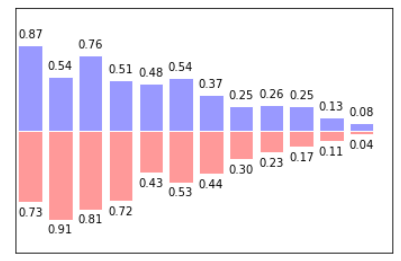
# 3.7.2 柱状图
import matplotlib.pyplot as plt
import pandas as pd
import numpy as np

n=12
X=np.arange(n)
Y1=(1-X/float(n))*np.random.uniform(0.5,1.0,n)
Y2=(1-X/float(n))*np.random.uniform(0.5,1.0,n)
plt.bar(X,+Y1,facecolor="#9999ff",edgecolor="white")
plt.bar(X,-Y2,facecolor="#ff9999",edgecolor="white")

for x,y in zip(X,Y1):
    plt.text(x,y+0.05,"%.2f" %y,ha='center',va="bottom")

for x,y in zip(X,Y2):
    plt.text(x,-y-0.05,"%.2f" %y,ha='center',va="top")

plt.xlim(-.5,n)
plt.xticks(())
plt.ylim(-1.25,1.25)
plt.yticks(())
plt.show()
1
2
3
4
5
6
7
8
9
10
11
12
13
14
15
16
17
18
19
20
21
22
2
3
4
5
6
7
8
9
10
11
12
13
14
15
16
17
18
19
20
21
22
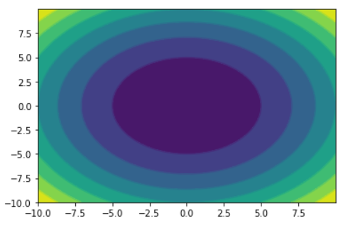
# 3.7.3 等高线
import numpy as np
import matplotlib.pyplot as plt

#建立步长为0.01,即每隔0.01取一个点
step = 0.01
x = np.arange(-10,10,step)
y = np.arange(-10,10,step)
#也可以用x = np.linspace(-10,10,100)表示从-10到10,分100份

#将原始数据变成网格数据形式
X,Y = np.meshgrid(x,y)
#写入函数,z是大写
Z = X**2+Y**2
#设置打开画布大小,长10,宽6
#plt.figure(figsize=(10,6))
#填充颜色,f即filled
plt.contourf(X,Y,Z)
#画等高线
plt.contour(X,Y,Z)
plt.show()
1
2
3
4
5
6
7
8
9
10
11
12
13
14
15
16
17
18
19
20
2
3
4
5
6
7
8
9
10
11
12
13
14
15
16
17
18
19
20
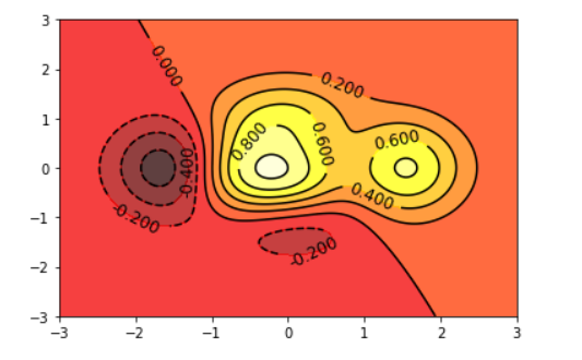
例二
import numpy as np
import pandas as pd
import matplotlib.pyplot as plt

# 计算x,y坐标对应的高度值
def f(x, y):
    return (1-x/2+x**5+y**3) * np.exp(-x**2-y**2)
# 生成x,y的数据
n = 256
x = np.linspace(-3, 3, n)
y = np.linspace(-3, 3, n)

# 把x,y数据生成mesh网格状的数据,因为等高线的显示是在网格的基础上添加上高度值
X, Y = np.meshgrid(x, y)

# 填充等高线
plt.contourf(X, Y, f(X, Y),8, alpha=0.75,cmap=plt.cm.hot)
# 添加等高线
C = plt.contour(X, Y, f(X, Y), 8,colors="black")
plt.clabel(C, inline=True, fontsize=12)
# 显示图表
plt.show()
1
2
3
4
5
6
7
8
9
10
11
12
13
14
15
16
17
18
19
20
21
22
2
3
4
5
6
7
8
9
10
11
12
13
14
15
16
17
18
19
20
21
22
# 3.8 图
# 3.8.1 图片
import numpy as np
import pandas as pd
import matplotlib.pyplot as plt

a=np.array([0.31,0.36,0.42,0.365,0.459,0.525,0.4237,0.5250,0.6515]).reshape(3,3)
plt.imshow(a,interpolation="nearest",cmap="bone",origin="upper")
# 添加图像
plt.colorbar()
plt.xticks(())
plt.yticks(())
plt.show()
1
2
3
4
5
6
7
8
9
10
11
2
3
4
5
6
7
8
9
10
11

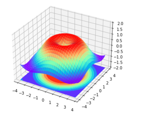
# 3.8.2 3D 图像
import numpy as np
import pandas as pd
import matplotlib.pyplot as plt
from mpl_toolkits.mplot3d import Axes3D
fig=plt.figure()
ax=Axes3D(fig)
X=np.arange(-4,4,0.25)
Y=np.arange(-4,4,0.25)
X,Y=np.meshgrid(X,Y)
R=np.sqrt(X**2+Y**2)
Z=np.sin(R)
ax.plot_surface(X,Y,Z,rstride=1,cstride=1,cmap=plt.get_cmap("rainbow"))

ax.contourf(X,Y,Z,zdir='z',offset=-2,cmap="rainbow")

ax.set_zlim(-2,2)
plt.show()
1
2
3
4
5
6
7
8
9
10
11
12
13
14
15
16
17
2
3
4
5
6
7
8
9
10
11
12
13
14
15
16
17
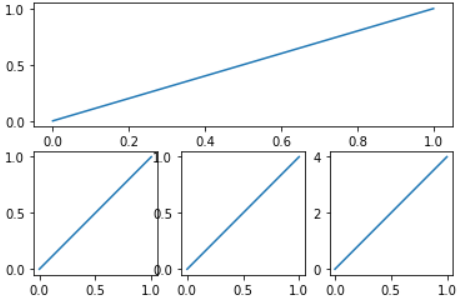
# 3.8.3 多图合一
import numpy as np
import pandas as pd
import matplotlib.pyplot as plt
plt.figure()

plt.subplot(2,1,1)
plt.plot([0,1],[0,1])

plt.subplot(2,3,4)
plt.plot([0,1],[0,1])

plt.subplot(235)
plt.plot([0,1],[0,1])
plt.subplot(236)
plt.plot([0,1],[0,4])

plt.show()
1
2
3
4
5
6
7
8
9
10
11
12
13
14
15
16
17
2
3
4
5
6
7
8
9
10
11
12
13
14
15
16
17
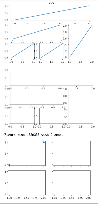
例二
import numpy as np
import pandas as pd
import matplotlib.pyplot as plt
import matplotlib.gridspec as gridspec

plt.figure()

# 第一种方法
ax1=plt.subplot2grid((3,3),(0,0),colspan=3,rowspan=1)
ax1.plot([1,2],[1,2])
ax1.set_title("title")

ax2=plt.subplot2grid((3,3),(1,0),colspan=2,rowspan=1)
ax2.plot([1,2],[1,2])

ax3=plt.subplot2grid((3,3),(1,2),colspan=1,rowspan=2)
ax3.plot([1,2],[1,2])

ax4=plt.subplot2grid((3,3),(2,0),colspan=1,rowspan=1)
ax4.plot([1,2],[1,2])

ax5=plt.subplot2grid((3,3),(2,1),colspan=1,rowspan=1)
ax5.plot([1,2],[1,2])
plt.show()

## 第二种方法
plt.figure()
gs=gridspec.GridSpec(3,3)
ax1=plt.subplot(gs[0,:])
ax2=plt.subplot(gs[1,:2])
ax3=plt.subplot(gs[1:,2])
ax4=plt.subplot(gs[-1,0])
ax5=plt.subplot(gs[-1,-2])
plt.show()

# 第三种方法
plt.figure()
f,((ax11,ax22),(ax21,ax22))=plt.subplots(2,2,sharex=True,sharey=True)
ax11.scatter([1,2],[1,3])
plt.show()
1
2
3
4
5
6
7
8
9
10
11
12
13
14
15
16
17
18
19
20
21
22
23
24
25
26
27
28
29
30
31
32
33
34
35
36
37
38
39
40
2
3
4
5
6
7
8
9
10
11
12
13
14
15
16
17
18
19
20
21
22
23
24
25
26
27
28
29
30
31
32
33
34
35
36
37
38
39
40
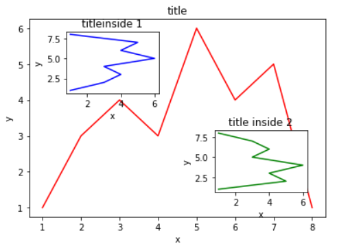
# 3.8.4 图中图
[x:y]为对列表取坐标为x到y的值,左边为闭区间取得到,右边为开区间取不到。
[x:y:z]为对列表取坐标为x到y的值,每间隔z个取1个值,同样为左闭右开,可以认为[x:y]是[x:y:z]的特例,其中z取1。
也可以输入负数:
[:-1]为剔除列表最后一个数字。
[::-1]为从列表最后一个开始取(即逆序),可以用a[::-1]取a的逆序。
[::-2]为从列表最后一个开始取(即逆序),每间隔2个取一次。
>>> a = [i for i in range(10)]
>>> a
[0, 1, 2, 3, 4, 5, 6, 7, 8, 9]
>>> a[0:3]
[0, 1, 2]
>>> a[0:3:1]
[0, 1, 2]
>>> a[0:3:2]
[0, 2]
>>> a[0:-1]
[0, 1, 2, 3, 4, 5, 6, 7, 8]
>>> a[0:0:-1]
[]
>>> a[::-1]
[9, 8, 7, 6, 5, 4, 3, 2, 1, 0]
>>> a[::-2]
[9, 7, 5, 3, 1]
1
2
3
4
5
6
7
8
9
10
11
12
13
14
15
16
17
2
3
4
5
6
7
8
9
10
11
12
13
14
15
16
17
例子
import numpy as np
import pandas as pd
import matplotlib.pyplot as plt
import matplotlib.gridspec as gridspec

fig=plt.figure()
x=[1,2,3,4,5,6,7,8]
y=[1,3,4,3,6,4,5,1]

left,bottom,width,height=0.1,0.1,0.8,0.8

ax1=fig.add_axes([left,bottom,width,height])
ax1.plot(x,y,'r')
ax1.set_xlabel("x")
ax1.set_ylabel("y")
ax1.set_title("title")


left,bottom,width,height=0.2,0.6,0.25,0.25

ax2=fig.add_axes([left,bottom,width,height])
ax2.plot(y,x,'b')
ax2.set_xlabel("x")
ax2.set_ylabel("y")
ax2.set_title("titleinside 1")


plt.axes([0.6,0.2,0.25,0.25])
plt.plot(y[::-1],x,'g')

plt.xlabel("x")
plt.ylabel("y")
plt.title("title inside 2")

plt.show()

print(y[::-1])
1
2
3
4
5
6
7
8
9
10
11
12
13
14
15
16
17
18
19
20
21
22
23
24
25
26
27
28
29
30
31
32
33
34
35
36
37
2
3
4
5
6
7
8
9
10
11
12
13
14
15
16
17
18
19
20
21
22
23
24
25
26
27
28
29
30
31
32
33
34
35
36
37
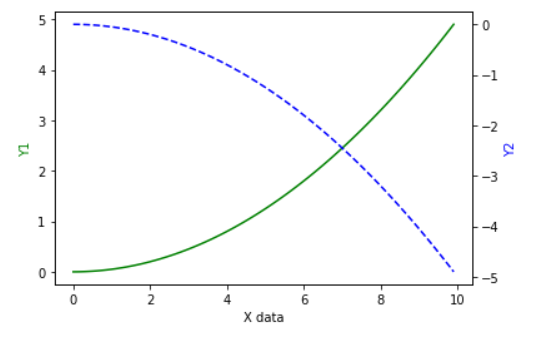
# 3.9 主次坐标轴
import numpy as np
import pandas as pd
import matplotlib.pyplot as plt

x=np.arange(0,10,0.1)
y1=0.05*x**2
y2=-1*y1
fig,ax1=plt.subplots()

ax2=ax1.twinx()
ax1.plot(x,y1,'g-')
ax2.plot(x,y2,'b--')
ax1.set_xlabel("X data")
ax1.set_ylabel("Y1",color='g')
ax2.set_ylabel("Y2",color='b')

plt.show()
1
2
3
4
5
6
7
8
9
10
11
12
13
14
15
16
17
2
3
4
5
6
7
8
9
10
11
12
13
14
15
16
17
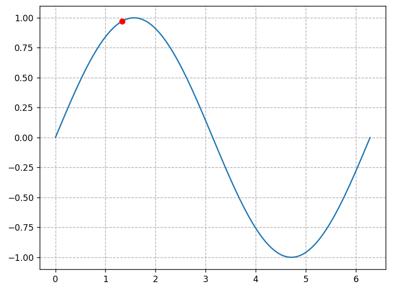
# 3.10 动画
import numpy as np
import matplotlib
import matplotlib.pyplot as plt
import matplotlib.animation as animation

# 指定渲染环境
%matplotlib notebook
# %matplotlib inline

def update_points(num):
    '''
    更新数据点
    '''
    point_ani.set_data(x[num], y[num])
    return point_ani,


x = np.linspace(0, 2*np.pi, 100)
y = np.sin(x)

fig = plt.figure(tight_layout=True)
plt.plot(x,y)
point_ani, = plt.plot(x[0], y[0], "ro")
plt.grid(ls="--")
# 开始制作动画
ani = animation.FuncAnimation(fig, update_points, np.arange(0, 100), interval=100, blit=True)

# ani.save('sin_test2.gif', writer='imagemagick', fps=10)
plt.show()
1
2
3
4
5
6
7
8
9
10
11
12
13
14
15
16
17
18
19
20
21
22
23
24
25
26
27
28
29
2
3
4
5
6
7
8
9
10
11
12
13
14
15
16
17
18
19
20
21
22
23
24
25
26
27
28
29
import numpy as np
import pandas as pd
import matplotlib.pyplot as plt
from matplotlib import animation

%matplotlib notebook

fig,ax=plt.subplots()

def animate(i):
    line.set_ydata(np.sin(x+i/100))
    return line,

def init():
    line.set_ydata(np.sin(x))
    return line,

x=np.arange(0,2*np.pi,0.01)
line,=ax.plot(x,np.sin(x))
ani=animation.FuncAnimation(fig=fig,
                            func=animate,
                            frames=100,
                            init_func=init,
                            interval=20,
                            blit=False)
plt.show()
1
2
3
4
5
6
7
8
9
10
11
12
13
14
15
16
17
18
19
20
21
22
23
24
25
26
2
3
4
5
6
7
8
9
10
11
12
13
14
15
16
17
18
19
20
21
22
23
24
25
26
